How To Apply Medianblur Filtering In Python

Goals

Larn to:

Mistiness images with various low pass filters
Apply custom-made filters to images (second convolution)

2D Convolution ( Image Filtering )

As in one-dimensional signals, images also can be filtered with various low-pass filters (LPF), high-pass filters (HPF), etc. LPF helps in removing noise, blurring images, etc. HPF filters help in finding edges in images.

OpenCV provides a function cv.filter2D() to convolve a kernel with an image. As an example, nosotros will try an averaging filter on an epitome. A 5x5 averaging filter kernel will await like the below:

\[K = \frac{1}{25} \begin{bmatrix} 1 & 1 & 1 & i & ane \\ one & 1 & one & i & 1 \\ ane & 1 & 1 & ane & 1 \\ 1 & one & 1 & 1 & ane \\ 1 & 1 & ane & 1 & 1 \finish{bmatrix}\]

The operation works like this: keep this kernel above a pixel, add together all the 25 pixels below this kernel, accept the average, and replace the central pixel with the new average value. This operation is continued for all the pixels in the image. Try this code and check the event:

            import            numpy            as            np
            import            cv2            equally            cv
            from            matplotlib            import            pyplot            as            plt
kernel = np.ones((5,5),np.float32)/25
plt.subplot(121),plt.imshow(img),plt.championship('Original')
plt.xticks([]), plt.yticks([])
plt.subplot(122),plt.imshow(dst),plt.title('Averaging')
plt.xticks([]), plt.yticks([])
plt.show()

Consequence:

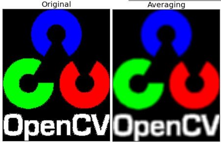
image

Epitome Blurring (Image Smoothing)

Image blurring is achieved by convolving the image with a low-laissez passer filter kernel. Information technology is useful for removing noise. It actually removes high frequency content (eg: noise, edges) from the prototype. So edges are blurred a lilliputian fleck in this operation (there are also blurring techniques which don't mistiness the edges). OpenCV provides four main types of blurring techniques.

one. Averaging

This is done by convolving an prototype with a normalized box filter. It simply takes the average of all the pixels nether the kernel area and replaces the central element. This is done past the office cv.blur() or cv.boxFilter(). Check the docs for more details well-nigh the kernel. We should specify the width and height of the kernel. A 3x3 normalized box filter would expect similar the below:

\[Yard = \frac{1}{ix} \begin{bmatrix} 1 & one & 1 \\ 1 & i & i \\ one & 1 & 1 \end{bmatrix}\]

Note: If you don't want to use a normalized box filter, utilise cv.boxFilter(). Pass an statement normalize=False to the function.

Check a sample demo below with a kernel of 5x5 size:

            import            cv2            every bit            cv
            import            numpy            as            np
            from            matplotlib            import            pyplot            as            plt
img = cv.imread('opencv-logo-white.png')
plt.subplot(121),plt.imshow(img),plt.title('Original')
plt.xticks([]), plt.yticks([])
plt.subplot(122),plt.imshow(blur),plt.championship('Blurred')
plt.xticks([]), plt.yticks([])
plt.testify()

Result:

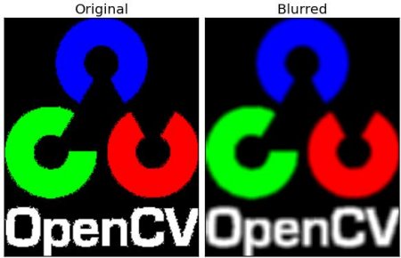
epitome

2. Gaussian Blurring

In this method, instead of a box filter, a Gaussian kernel is used. It is done with the function, cv.GaussianBlur(). Nosotros should specify the width and height of the kernel which should be positive and odd. Nosotros also should specify the standard deviation in the X and Y directions, sigmaX and sigmaY respectively. If simply sigmaX is specified, sigmaY is taken as the aforementioned as sigmaX. If both are given equally zeros, they are calculated from the kernel size. Gaussian blurring is highly effective in removing Gaussian noise from an image.

If y'all want, you lot can create a Gaussian kernel with the office, cv.getGaussianKernel().

The above code can exist modified for Gaussian blurring:

Outcome:

image

3. Median Blurring

Here, the function cv.medianBlur() takes the median of all the pixels nether the kernel area and the central element is replaced with this median value. This is highly effective against common salt-and-pepper racket in an prototype. Interestingly, in the in a higher place filters, the central element is a newly calculated value which may be a pixel value in the prototype or a new value. But in median blurring, the central element is always replaced by some pixel value in the paradigm. It reduces the dissonance finer. Its kernel size should exist a positive odd integer.

In this demo, I added a 50% noise to our original prototype and practical median blurring. Check the result:

Result:

image

4. Bilateral Filtering

cv.bilateralFilter() is highly effective in dissonance removal while keeping edges sharp. Only the operation is slower compared to other filters. Nosotros already saw that a Gaussian filter takes the neighbourhood around the pixel and finds its Gaussian weighted average. This Gaussian filter is a function of space lone, that is, nearby pixels are considered while filtering. It doesn't consider whether pixels accept almost the same intensity. It doesn't consider whether a pixel is an edge pixel or not. So it blurs the edges likewise, which we don't desire to do.

Bilateral filtering also takes a Gaussian filter in space, simply ane more Gaussian filter which is a function of pixel deviation. The Gaussian function of space makes sure that simply nearby pixels are considered for blurring, while the Gaussian function of intensity difference makes certain that simply those pixels with similar intensities to the central pixel are considered for blurring. Then it preserves the edges since pixels at edges volition have big intensity variation.

The below sample shows employ of a bilateral filter (For details on arguments, visit docs).

Result:

image

See, the texture on the surface is gone, simply the edges are nonetheless preserved.

Boosted Resource

Details virtually the bilateral filtering

Exercises